What is the downside risk for US equities?

A lot of people make decisions on how to allocate their investments between markets based on their assessment of the most likely return from each market, but it is comparatively rare for people to think deeply about worst case scenarios when making asset allocation decisions. This is potentially an oversight, as perhaps the best way to evaluate your tolerance for risk is to think about how you would be affected by the worst (or almost-worst) possible outcome for the portfolio you are considering.

In this column, I will try to evaluate an “almost worst-case scenario” for returns from the US equity market. I will look at this from two perspectives: firstly, the downside risk implied by the month-to-month volatility of the US equity market; and secondly, by making an assessment of what fundamentals (and their history) tells us about the potential downside for the US market.

In looking at downside risk, I’m trying to identify a return that represents about a one-in-twenty (i.e 5%) probability. Of course, there is always a small chance of far worse scenarios (for example, it is not impossible to imagine that the stable genius currently in charge of the United States could suddenly decide that it’s in America’s interest to seize ownership of all foreign-owned US assets), but I think it is more meaningful to think about whether there is a 5% chance of -50%, returns rather than worrying too much about whether there’s a 0.5% chance of -100% returns. Either scenario could damage a lot of retirement plans, but the former is more likely.

Estimating Downside Risk based on volatility of Return

The most common approach from sophisticated asset allocators is to make asset allocation decisions in the context of the combination of expected return and risk. Although this approach does not incorporate explicit consideration of a “worst case” scenario, it does incorporate an implicit evaluation of downside.

“Expected return” represents the average of all possible future returns (typically over a time horizon of a decade or more). The expected return should in theory be slightly higher than the median of all possible returns. However, when we forecast future returns using fundamental approaches like “dividends plus growth”, it’s not always clear whether our forecast return is best thought of as an estimate of “expected return” or “most likely return”.

“Risk” is typically measured as the annualised standard deviation of returns, using the variability of returns over relatively short time intervals such as monthly returns. If markets follow a random walk, then the volatility of returns over short time periods should theoretically provide a reliable estimate of the potential variability of returns over longer time periods such as a decade. Hence, the standard asset allocation approach implicitly assumes that potential divergence of actual returns from expected returns over the long-term is proportionate to the standard deviation of short-term returns.

If we look at the volatility of US equity markets over the past 10, 20, or 30 years, we see a monthly standard deviation of return of about 4.45%, which converts to an annualised standard deviation of 15.5%. Looking at expected return, I have argued in previous columns that it is reasonable to assume a long-term return from the US equity market of about 7% per annum.

Using these starting points for risk and expected return, we can calculate the potential distribution of future returns if markets follow a random walk. If markets follow a random walk, then the distribution of potential future returns should theoretically follow a positively-skewed lognormal distribution. As an example, in the graph below I show the theoretical distribution of US equity market returns over the next decade.

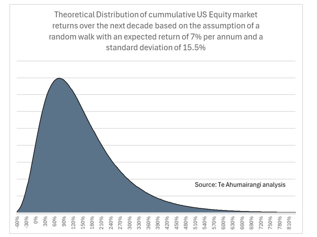
I defined my “almost-worst-case scenario” as being a return for which there was only a 5% probability that returns could be even worse. Statistically, this represents an outcome that is 1.64 standard deviations below the mean. Based on an assumption that the market follows a random walk with a volatility similar to what we’ve seen over the past 30 years (around expected returns of 7% per annum returns), we can calculate the following “almost worst case” scenarios for US equity returns, shown in the middle column of the table below:

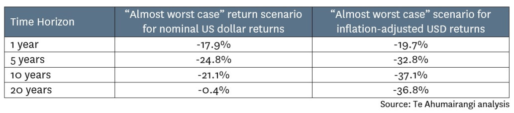
In the right column, I show what the worst case scenario looks like in inflation-adjusted terms. While the middle column makes it seem like a 20-year horizon is sufficiently long to virtually eliminate any chance of losing significant money in US equities, the right column suggests that this mainly an illusion created by inflation. In inflation-adjusted terms the potential loss over 20 years is still greater than 35%.

Of course, the analysis behind this table is reliant on the assumption that markets follow a random walk. While the month-to-month behaviour of global equity markets seems to be a very close approximation of a random walk (the correlation between returns in one month and returns in the next month has been less than 0.01 over the past 30 years), this does not necessarily mean that monthly volatility in returns is necessarily the best estimator of how much potential variation in returns investors could expect over much longer periods of time.

In fact, at least 3 observations make me believe that the random walk is not a particularly accurate model for understanding how equity markets may perform over longer time periods of a decade or more:

1. Looking back through financial history, there have been numerous incidents when equity markets have declined by much more than would seem possible based on the modest volatility of equity markets in the years prior to each “crash”.
2. There has historically been an inverse relationship between returns over one ten-year period and returns over the following ten-year period. This suggests that there is some tendency for equity markets to revert over longer time periods.
3. The historical distribution of ten-year returns from equities does not show any evidence of the positive skew that we should expect if equity markets truly followed a random walk.

So, although the random walk is the favoured model for many academics, given its failure to adequately explain historical patterns in long-term equity market returns, I think it is important to also think about what market fundamentals may tell us about downside risk in the US equity market.

Estimating Downside Risk based on History & Market Fundamentals

From a fundamental perspective, we can think of each equity market as being valued at a multiple of its annual earnings power. Accordingly, downside in the US equity market could occur due to either declines in corporate earnings and/or a reduction in earnings multiples.

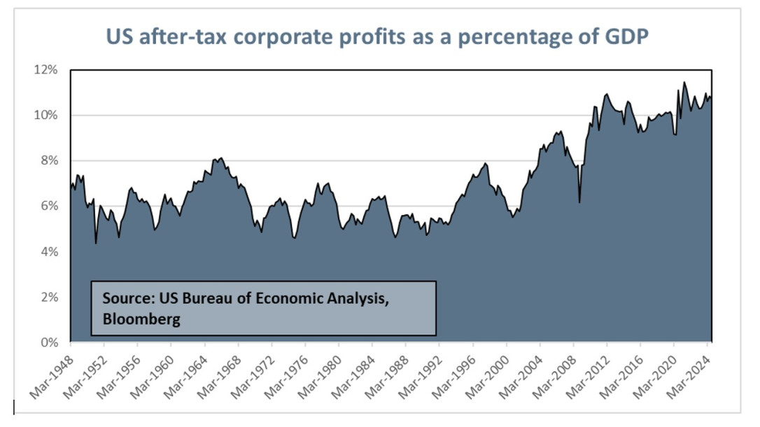
The graph below shows the history of US corporate profits measured as a percentage of US GDP. As can be seen, the current level of corporate profitability is (at 10.7% of GDP) is close to all time highs. Historically, corporate profits have sometimes dipped below 5% of GDP, and have stayed at around 5.5% of GDP for sustained periods of time. Hence, an almost-worst-case scenario would seem to be that the profit/GDP ratio could halve from current levels.  

While a starting assumption might be that US corporate profits grow in line with nominal GDP at about 4.5% per annum (translating into about 4% per annum growth in the earnings per share of US listed companies), the risk of a halving in the ratio of corporate profits-to-GDP means that a downside scenario is that earnings per share could be 26% lower in 10 years’ time than they are today, even if GDP continued to grow at 4.5% per annum.

After allowing for the likelihood that a slump in profitability (and the equity market) would be associated with a US recession, it seems reasonable to assume that in the almost-worst-case scenario, US GDP would not grow at 4.5% per annum, and earnings per share for the US market could therefore fall 29% over the course of a decade.

The other thing we need to think about is what price/earnings multiple the US equity market could trade at in the future. The US equity market currently values listed companies in aggregate at about 25.5 times the earnings per share they generated over the course of 2025. As we can see in the graph below, this is towards the upper end of the historical range, as the US equity market has historically traded mainly in a range of between 13 and 28 times trailing earnings per share.

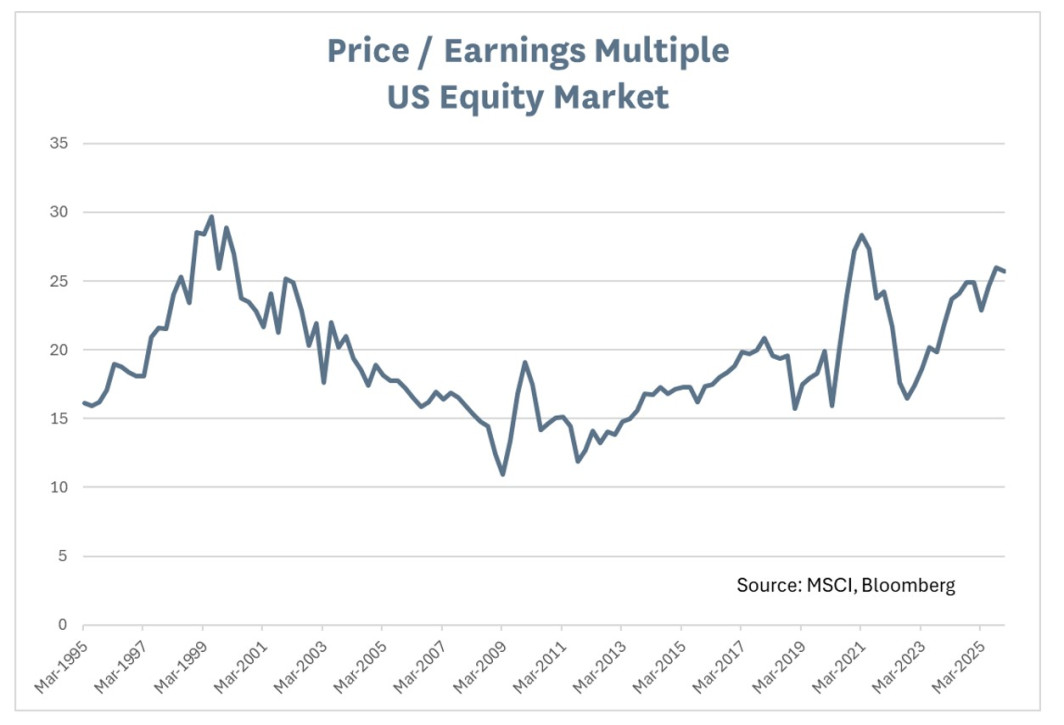
Since the purpose of this exercise is to consider an “almost worst case” scenario, we must consider what would happen to equity prices if the P/E multiple declined towards the lower end of its historical range. In isolation, a decline in the P/E multiple from its current level of about 25.5 to a near-low of 13.0 would reduce the value of the US equity market by 49%.

When we combine the possibility of a 29% decline in earnings per share over the next decade with the possibility of a 49% decline in the price/earnings ratio of the US equity market, a 64% decline in nominal US equity prices seems possible as a near-worst-case scenario.

One objection to this calculation might be an expectation that price/earnings multiples may tend to compensate for fluctuations in earnings, by rising when earnings are temporarily depressed and falling when earnings are temporarily inflated. While this expectation seems reasonable, it is not in fact supported by the historical evidence. If anything, there has actually been a slight positive correlation between earnings levels and price/earnings multiples over the past 40 years.

A 64% decline in US equity prices would translate to a 10-year cumulative US dollar return from the US share market of about -52%, as dividends would improve the total return. This is obviously worse than the -21% return that we derived by simply assuming a random walk.

Adjusted for inflation, a -52% return from US equities over the next decade would represent a roughly 62% loss of US dollar purchasing power for an investor in US equities.

Conclusions

US equities currently carry an unusually high level of risk, because they are valued at an unusually high multiple of earnings per share, and because earnings are at historically high levels as a proportion of GDP. There is at least some risk that both P/E multiples and corporate earnings levels could decline from their current highs, towards levels that are closer to historical lows.

If this happens, the average US equity portfolio could lose about 52% over the next decade, representing a 62% loss of purchasing power after taking account of inflation.

Such losses could have a major impact on some global equity portfolios, which in many cases have as much as 75% of total assets invested in the United States. Such a severe decline in the value of the US equity market would likely result in losses of much greater than 52% in growth-orientated US equity portfolios, as growth stocks tend to fall by more than the broader market in most market downturns.

I should emphasise that the point of this exercise was to evaluate the potential downside risks for the US equity market, and the fact that I can see the possibility of such large losses over the next 10 years does not imply that I actually believe that such losses are likely. Rather, my central expectation is that the US equity market will deliver positive returns over the next decade (although I don’t expect these returns to be as strong as the returns that I would expect from other global equity markets).

However, I consider it important that both investors making decisions about allocating funds to US or global equities, and fund managers managing portfolios of global equities, do so with an awareness of the downside risks.

 

Nicholas Bagnall is Chief Investment Officer of Te Ahumairangi Investment Management

Disclaimer: This article is for informational purposes only and is not, nor should be construed as, investment advice for any person. The writer is a director and shareholder of Te Ahumairangi Investment Management Limited, and an investor in Te Ahumairangi Global Equity Fund. Te Ahumairangi manages client portfolios (including Te Ahumairangi Global Equity Fund) that invest in global equity markets.