Paradoxes & pitfalls of measuring average returns

Over the past 6 calendar years, the arithmetic average annual return from bitcoin has been 78.9% when measured in US dollars.

Over the same 6-year period, the arithmetic average annual return from the MSCI World index (an index measuring the returns from developed market global equities) has been 11.0% when measured in US dollars.

If we momentarily accept the position of some bitcoin devotees that bitcoin is the one true currency that everything else should be measured in terms of, perhaps we should measure the average return from the MSCI World index in terms of bitcoin.

So, what do think that the arithmetic average return from the MSCI World index has been over the past 6 years when measured in terms of bitcoin?

I would hazard a guess that many readers will presume that since the average annual return from bitcoin has been so much higher than the average return from the MSCI World index over the past 6 years, the arithmetic average return of the MSCI World index must have been negative when measured in terms of bitcoin.

However, this presumption is incorrect. The arithmetic average annual return of the MSCI World index has actually been a whopping +33.8% when measured in terms of bitcoin over the past 6 years. This can be seen in the table below:

 Arithmetic average returns are calculated by simply calculating the average of the annual returns in the table above. An alternative approach is to calculate geometric average returns (a.k.a. “compound returns”) by working out what constant rate of return would have delivered the same cumulative return that investors would have received if they’d had all their money invested in that asset over the full period.

Investing from Bitcoin Land

While the table above showed that the arithmetic average return from the MSCI World index had been negative when measured in bitcoin, a native resident of “Bitcoin Land” (presumably with a consumption basket consisting mainly of “dark web” purchases) would no doubt observed that cumulative returns from the MSCI world index have been pretty awful over the past 6 years when expressed in their preferred “currency”. The MSCI World index delivered a compound average return of -8.7% per annum over these 6 calendar years when measured in bitcoin.  This negative compound average return means that if a resident bitcoiner had invested all their bitcoin into the MSCI World index, they would have been 42.2% worse off than if they’d just kept all their bitcoin stuffed under their digital mattress*.

* Contingent on that “digital mattress” not being one of the numerous crypto exchanges that gone bust over the last few years.   

Looked at from this perspective, expressing returns in terms of arithmetic averages seems to be just a form of mathematical trickery, which makes volatile returns look better than they actually are. In large part, I’d agree with this assessment, but it is also worth looking at how Bitcoin Land domiciled investors could have benefitted from the high arithmetic average returns, even though cumulative returns from the MSCI World index were negative:

Consider how our hypothetical resident of Bitcoin Land would have fared if they’d invested a modest percentage of their bitcoins into the MSCI World index while leaving the rest in bitcoin, and followed a strict policy of rebalancing back to the same percentage mix between the MSCI World index and bitcoin at the end of each year.

For this example, let’s assume that the resident bitcoiner started off with 100 bitcoins at the end of 2017, and followed a policy of allocating 20% of their financial wealth to global equities (as proxied by the MSCI World index) each year. Following this policy, they would have put 20 of their bitcoins into the MSCI World index at the end of 2017 (while leaving the other 80 bitcoins under the mattress). As a consequence of this 20% allocation to global equities, they would have enjoyed a 50.1% return over 2018 (i.e. 20% of 250.5%), lifting the value of their portfolio to 150.1 bitcoins. Continuing with this policy, they would have rebalanced their portfolio at the end of 2018 so that 20% (i.e. 30 bitcoins) was invested in the MSCI World index and the other 120.1 bitcoins were stuffed under the mattress. This would have resulted in a loss -6.6% (20% of -32.8%) over 2019, and so on (see table below). By the end of 2023, this resident Bitcoiner would have been 29.8% better off due to investing 20% of their financial wealth in global equities than would have been the case if they’d left everything in bitcoin for the entire period.     

Hypothetical investment portfolio of a resident of “Bitcoin Land”

 Arithmetic average vs geometric average (compound) returns

For relatively stable investments measured in terms of a relatively stable currency, there is typically only a small difference between arithmetic average returns and compound returns. For example, the Te Ahumairangi Global Equity fund has been relatively stable (with an annualised standard deviation of monthly returns of just 7.7%), and its annualised average monthly return since inception (11.75%) only slightly exceeds the annualised compound return since inception (11.47%).

However, when you look at more volatile investments, a large gap can open up between arithmetic average returns and geometric average returns, as we can see from the example of bitcoin shown in the first table in this article. Bitcoin may boast a 78.9% arithmetic average return over the past 6 calendar years, but the compound average return was far more modest, at 19.9%.

As a rough rule of thumb, average returns will typically exceed compound returns by about half of the standard deviation squared. So: for investments with standard deviation of 10%, we will typically find that arithmetic average returns are about 0.5% higher than geometric average returns (calculated as 50% of 10% of 10%); for investments with standard deviations of 20%, this gap increases to 2.0% (50% of 20% of 20%); and for investments with standard deviation of 30%, the gap between the two measures of average return will typically be about 4.5% (50% of 30% of 30%).

Different returns for different purposes

Which measure of average return is best to use depends on the purpose for which you are using the returns. Arithmetic average returns are always higher than geometric average returns, and for this reason there is a real risk that the use of arithmetic average returns could lead to an over-estimation of the central tendency for returns. Accordingly, it you are trying to assess the performance of a complete investment strategy or an investment fund, it makes more sense to look at compound average returns than arithmetic average returns. Consistent with this, New Zealand’s Financial Markets Conduct Regulations require that fund managers report their funds’ returns in terms compound average returns.

However, arithmetic average returns are widely used by finance academics and quantitative stock pickers. Why is this?

One key reason why finance academics may prefer to look at arithmetic average returns rather than geometric average returns is that arithmetic average returns are conceptually consistent with metrics already used in finance theory. Measures such as standard deviation and beta are calculated based on divergences from arithmetic average returns (not geometric average returns) and the arithmetic average return of a portfolio can be calculated from the weighted average of the arithmetic average returns of the stocks within the portfolio, but the same cannot be said for compound average returns.

A reason why quantitative fund managers look at arithmetic average returns rather than geometric average returns will be that they like to layer many different quantitative screens together when selecting stocks, such that no single quantitative screen will have a huge impact on the overall shape of their portfolios. If a quantitative manager is studying how one extra screen could contribute in a small way to the shape of their portfolios, it makes more sense for them to look at the arithmetic average returns from the strategy rather than compound average returns.

However, selecting stocks based on quantitative criteria that have historically generated strong arithmetic average returns can contribute to a bias towards risk-taking on the part of quantitative managers, and can cause them to overlook screens that favour stocks with favourable risk characteristics.

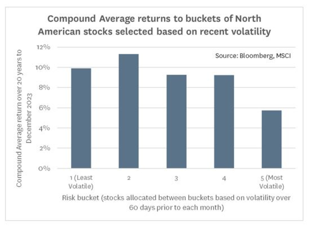
As an example of this, I have used the Factor Backtester on Bloomberg to run a back-test looking at the returns you would get from large- and mid- capitalisation North American stocks if you divided them into different buckets each month based on the volatility that you would have seen in their share prices over the preceding 60 days.   

Based on the data shown in the graph above, your average quantitative manager or finance academic might conclude that recent volatility hasn’t been a particularly useful tool for selecting stocks, as on average, the returns from each risk bucket have been fairly similar (albeit with a slightly lower return to the most volatile stocks) over the past 20 years.

However, the picture changes if we present the results of the same back-testing in terms of the compound average returns you would have got from each bucket of stocks. Using this perspective, there is a clear inverse relationship between recent volatility and subsequent return, with the most volatile quintile of stocks delivering compound returns over the past 20 years that have been more than 4% per annum worse than returns from the least-volatile and second-least-volatile quintiles of stocks.    

By using models that select stocks based on arithmetic average returns rather than geometric average returns, quantitative fund managers can sometimes end up crowding into the stocks where returns are most overstated by the use of arithmetic average returns. Quant models optimised based on arithmetic average returns will sometimes plunge into volatile “exciting” stocks like Tesla and Gamestop that are already overcrowded due to how speculative punters similarly get captivated by the excitement of volatile share prices.

Arithmetic average returns and “expected returns”

One reason why academic finance writing tends to focus on arithmetic average returns is that they conceptually similar to “expected returns”, a concept that is used widely in finance theory. Conceptually, expected returns are defined as the weighted average of all possibilities, rather than simply the most likely scenario. Thinking about the weighted average of all possibilities makes a lot of sense if (for example) you are considering a subordinated debt instrument that you think has a 99% probability of delivering you a return of 8% (if everything goes according to plan) and a 1% probability of delivering you a return of -100% if the issuer goes bust. In this case your “expected return” would be 6.92% (calculated as the sum of 99% of 8% and 1% of -100%). Mathematically, calculating an expected return that is a weighted average of all possibilities is very similar to calculating the simple average of the returns that an investment has delivered over a series of months or years.

However, this concept of “expected returns” differs from the prospective returns that long-term investors will typically contemplate when we think about the returns that an investment security may deliver over several years. For example, at Te Ahumairangi, we typically model a company’s financial outlook to forecast the cashflows that we expect it to deliver to shareholders over the next 15 years and also forecast a middle-of-road expectation of what that company will be worth in 15 years’ time. We use these numbers to calculate a projected internal rate of return from investing in the company. This approach to estimating future return is more aligned with the concept of compound average returns than with arithmetic average returns.

But shorter-term more speculative investors may think about future returns in a way that is more conceptually similar to arithmetic average returns, weighing up different scenarios for a share price over the next year. In doing so, they run the risk of being lured by the same upward bias that is apparent in the calculation of arithmetic return.

As an extreme example of this, let’s return to bitcoin. I am personally of the view that bitcoin will most likely end up being worthless within my lifetime, but using the concept of expected returns, I might still calculate positive expected returns in each individual year, given the extreme volatility in the price of bitcoin. For example, I might express a simplified version on my expectations for the potential future return distribution of bitcoin by saying each year there is a 50% chance that it will rise by +120% and a 50% chance that it will fall by -80%. The expected return from the combination of these two scenarios is +20% (50% x -80% + 50% x +120%), which is significantly higher than the returns that I would expect from most other investments.

However, logic also implies that (under my world-view) the most likely scenario over the next 20 years is that we’ll see 10 individual years when bitcoin falls by -80% and 10 individual years when it rises by +120%. The cumulative outcome of this scenario generates a central expectation that bitcoin will most likely fall by -99.97% over 20 years (a compound average return of -33.7% per annum).

There’s a paradox here, in that investors can rationally assess high “expected returns” from speculative “investments” that they ultimately expect to go to zero. If they have a high risk tolerance and construct portfolios based on short-term expected returns, they could end up invested in “greater fool theory” portfolios that they know will probably ultimately be worthless, but hope to sell to someone else before the party ends.

Siegel’s Paradox

Another consequence of the upward bias in arithmetic average returns and “expected returns” is that it is possible for an American and a New Zealander to have identical world views but to both simultaneously expect that they can enhance the return of their investment portfolios over time by including a modest portion of unhedged exposure to the other’s currency within their investment portfolios. For example, consider the table below, showing the returns that NZ investors have got from US dollar exposure and the returns that US investors have got from NZ dollar exposure over the past 20 years.

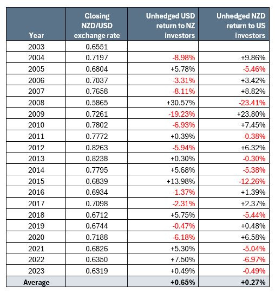
Source: Bloomberg

On average, investors in each country would have benefitted from a bit of exposure each year to the other’s currency (although for the New Zealander, the forward point pick-up from hedging US dollar exposure would have been even better). Obviously, as the New Zealand dollar has fallen slightly against the US dollar over the 20-year period, the US investor would not have benefited if they’d had their entire portfolio invested in NZ dollar investments throughout the period, but if they’d had a small unhedged exposure to NZ dollars (say 10% of their investment portfolio), and rebalanced this back to 10% each year, they would have seen the benefit of positive average return from NZ dollars when expressed in USD.

This effect is known as “Siegel’s paradox”, after Jeremy Siegel, who first highlighted it.

Could investors benefit from a lot of small exposures to volatile investments?

In this article, I hope I’ve shown you that while the difference between arithmetic average returns and geometric average returns is partly mathematical trickery, there is also an element of truth to it, which investors can sometimes exploit in a modest way.

The “true” aspect of:

(1)     volatility boosting arithmetic average returns; and

(2)    this volatility contributing to overall portfolio performance if investors take their exposures in small doses

may naturally lead investors to wonder whether they could build up portfolios consisting of small exposures to a large number of very volatile investments, and hope that a significant proportion of these volatile investments will come right each year.

For example, let’s use my previous example a potential the return distribution for bitcoin, where I hypothesised a 50% chance of a -80% return and a 50% chance of a +120%. Imaging that you could find 100 different investments that looked like this, and invest 1% of your portfolio in each of them. In theory, you might expect about 50 of them to return -80% each year and 50 of them to return +120%, and therefore anticipate an aggregate return of about +20% each year.

However, in order for this idea to work, you’d need to be reasonably confident that you wouldn’t strike any years when a large proportion of these individually risky investments delivered the “bad return” of -80%. You could rule this possibility out if the different investments were uncorrelated, but the harsh reality of the real world is that most risky investments are highly correlated to each other. They rise together when people are chasing speculative investments, and they decline in unison when speculative bubbles deflate.

You can see this correlation in action if you look back to the first table in this article, where I showed the annual returns of both bitcoin and global equities. In the “good years”, bitcoin delivered returns that were on average about 6 times as high as the returns from global equities, but in the “bad years” it delivered losses that were also about 6 times as large as the losses on global equities. The valuations of global equities are clearly affected by the “animal spirits” of investors and speculators, but bitcoin is hyper-sensitive to these animal spirits.

You will see the same patterns of returns from other volatile investments that have attracted a lot of speculative activity, such as the meme stocks and the growthiest technology stocks. In short, it is very difficult to find volatile investments that are not strongly correlated to other volatile investments. Even when you do spot a volatile investment that seems to be uncorrelated to other volatile investments, it often seems to transpire that that investment suddenly becomes highly correlated with the next market crash.

Hence, the theory that you might be able to get the benefit of volatility enhance arithmetic average returns whilst somehow diversifying away the risk does not generally work out in practice. Gold and gold-mining stocks might be a small exception to this rule, as they tend to be volatile yet have remained relatively uncorrelated to global equities over long periods of time. Another exception for NZ-based investors is that the positive expected return from unhedged foreign currency exposure arising from volatility in the NZ dollar is not positively correlated to returns from other risky assets, as the NZ dollar counts as a “risky asset” in the eyes of investors in other parts of the world, and for this reason unhedged currency works out as a hedge against the downside of global animal spirits for those of us fortunate enough to be looking at the NZ dollar from the “other side of the mirror”.     

Nicholas Bagnall is chief investment officer of Te Ahumairangi Investment Management

Disclaimer: This article is for informational purposes only and is not, nor should be construed as, investment advice for any person. The writer is a director and shareholder of Te Ahumairangi Investment Management Limited, and an investor in the Te Ahumairangi Global Equity Fund. Te Ahumairangi manages client portfolios (including the Te Ahumairangi Global Equity Fund) that invest in global equity markets.